Speech recognition 101: Hands on Keyword Spotting 2/3
This 3-part tutorial series will take you on an adventure to build your own neural network keyword spotter with step-by-step lecture and coding exercises. Part two will discuss the training of neural networks for audio classification.
 source: Pixabay
The tutorial series
Automatic Speech Recognition (ASR) is the task of translating speech to text. A full fetched ASR system is very powerful and has a wide range of applications. However, building such systems usually requires expert knowledge, large datasets and computational resources. Consequently, the topic is hard to access for beginners. Meanwhile Keyword Spotting (KWS) is the task of recognizing a limited set of keywords from speech. While conceptually similar, building decent models requires less data, computing time and less expert knowledge. Therefore, it is the ideal starting point for learners and we will build a keyword spotter from scratch, in the following three tutorials:
-
Audio: preprocessing data for speech recognition tasks
-
Machine Learning: training neural networks for keyword spotting
-
Application: Building an app to deploy the model in a Jupyter Notebook
The code and exercises were designed for the audio track of ML summer school at University of Cologne and every article will have theory input followed by practical exercises, that can be downloaded from this repository.
The big picture
The big picture of the keyword spotter is shown below. We have dealt with the Feature Extractor in the first part of the series and will now go towards the center piece of the application: The classifier.
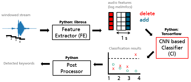 Figure 1: big picture of the keyword spotting application.
While there are many possibilities, we will realize the keyword spotter as a classifier that predicts probabilities for certain words being present in a window of a fixed length of one second. Instead of words one could use phonemes, sub-words, or characters instead, each with their own advantages and disadvantages.
Part 1: Audio classification for keyword spotting
We want to train a classifier that gets a time series of MFCCs as an input and returns several class probabilities, one class representing one keyword. In the exercises the keywords will e.g., be yes, no, unknown, silence and so on. Let’s revisit the most important concepts for machine learning and classification tasks in particular.
Machine Learning cycle
The typical steps in Machine Learning include:
-
Data gathering: Done. This is already done for us. We will use the Google-Speech-Commands dataset. It contains a large collection of roughly one-second long utterances, that contain one keyword each. We will extract MFCCs and create one-hot encoded labels for each utterance in the exercises.
-
Feature engineering: Done. We have discussed this extensively in the last tutorial. We will use MFCC features, that are proven to work well for speech recognition
-
Training: up next. We will want to train several (deep neural) models.
-
Evaluation: up next. We need suitable metrics to evaluate the quality of our models.
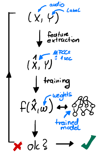 Figure 2: Machine Learning cycle.
Model architecture
We will train a classifier that predicts which keyword (class) is present, from the MFCC features of a one-second long audio clip. Let’s discuss the models’ basic architecture.
Input: The MFCCs of an audio signal are similar to a grayscale image, where the (x,y) plane corresponds to time and MFCC coefficient, respectively. The intensity value corresponds to the value of the coefficient. That leaves us with a (T,F) sized input matrix of real values. Regarding the structure of the connections between the neurons, there are multiple possibilities, where the simplest is a Feed Forward Neural Network. Since a FFNN expects one dimensional input, we can write the (T,F) MFCC output into one vector. This is the simplest possible structure and we will start with it in the practical exercises.
Output: The network should output class probabilities for each keyword. To achieve these outputs, we will choose a softmax activation function for the last layer:
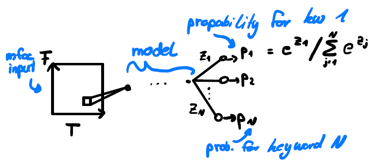 Equation 1: network structure with MFCC input and probabilities for each class as output.
where z_i is the value going into the softmax function and p_i the output for class i that the neural network produces. This has the property that the sum over all output values is 1 and that every output value is between 0 and 1 and can be interpreted as the probability of a particular class being present in the audio.
Dataset
To train the classifier we use the Google Speech Commands dataset. It contains one-second-long recordings of different keywords like “yes”, “no”, ”up”, “down” etc. from roghly 2600 different speakers. We will use the 10 keywords that have between 3500 and 4000 recordings each and create a “unknown” class from the remaining keywords. Furthermore, we add a “silence” class, which yields a total of 12 classes corresponding to 12 output neurons of our classifier. We will explore the dataset during the next exercise.
Evaluation of classification tasks
In supervised deep learning the training algorithm usually tries to find local minima of the loss function f, by optimizing the model parameters w the loss function depends on. In our case we use the Categorical Entropy loss, which is the log likelihood of the training dataset being classified correctly:
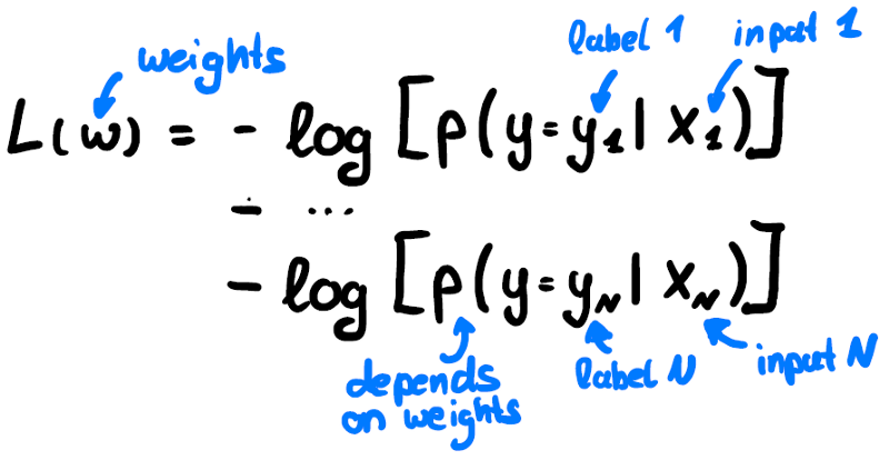 Equation 2: Loss of the training set.
It is 0 if the likelihood of classifying each instance in the training set correctly, is 1. While this is a great metric for the optimization problem that is solved in the background during training, it is more useful to use a different metric to judge how well our model works in real life. Therefore, it is useful to consider the possible cases when classifying an instance:
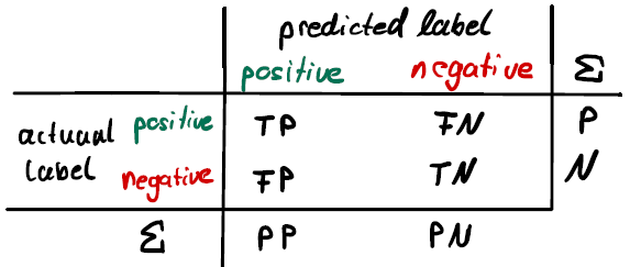 Figure 3: classification. TP: True Positive, FN: False Negative and so on. PP/PN stands for Predicted Positive/Negative. P/N stand for the total number of Positive/Negative events, respectively.
Now when evaluating on a test dataset one can simply classify all instances and add up to obtain the total number of TP, FN, FP, TN events. From it one can calculate several metrics:
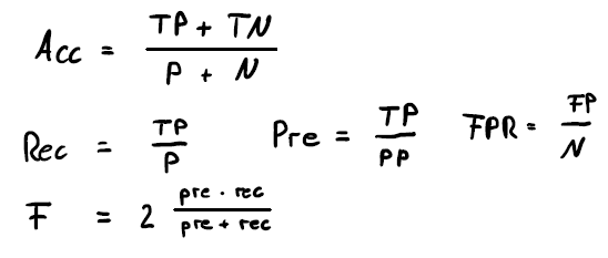 Equation 3: various classification metrics are shown.
The accuracy (Acc) describes how often the classification was correct and is the simplest and most intuitive measure. It is useful but also has some limitations. Imagine there are many more positive than negative examples in a series of tests. Then classifying all seen events as positive yields a great accuracy but we did not learn anything. Also, it does not distinguish what kind of errors were made. Therefore, it is often better to look at a pair of metrics like precision (Pre) and recall (Rec)/true positive rate (TPR) or TPR and false positive rate (FPR). Another possibility is using the F score, a measure that combines both into one metric. Which pair of metrics to choose depends on the Use Case.
We can use this pair of metrics now to judge the classifier quality. Let’s go back to the neural network output to understand how: Since the output of our neural network will be probabilities, one needs to define a threshold over which we accept the occurrence of a keyword (or equivalently a positive test in our example). The simplest case would be p>1/N, where N is the number of classes. However, by increasing that threshold we can tradeoff between e.g. FPR and FNR, which is highly relevant. Say we have a Covid test and accepted only tests as positive that have a probability of 1. This would yield a great FPR while causing a terribly high FNR. If we accepted all tests with a probability higher then say p>0.5, we would get a great FNR but a high FPR instead. That example shows that our test is a curve in the TPR-FPR (or equivalent pair of metrics) plane:
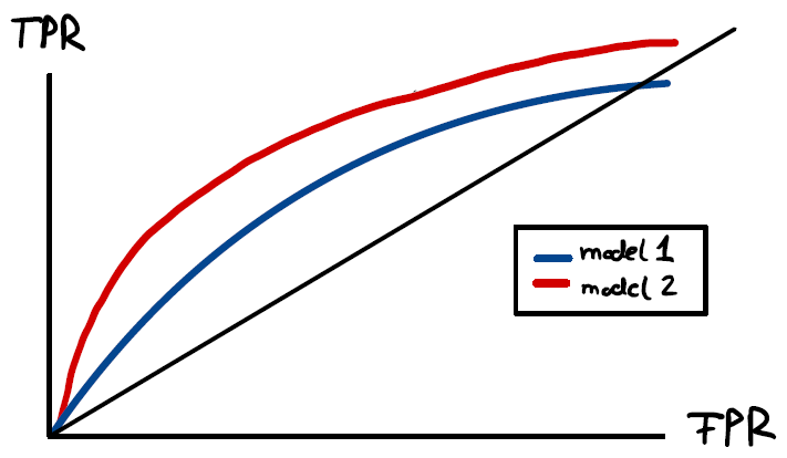 Figure 4: example ROC curves.
We can compare different models now by these so-called ROC curves. In Figure 4, the red model is better than the blue one, since at every given FPR it has a higher TPR. This is also reflected in the higher area under the red curve, which is an often-used classification metric as well.
Another very useful tool when it comes to evaluating classifier performance is the confusion matrix. We simply create a matrix where the rows stand for the actual class label and columns for the predicted class label. Then, for each classification in the test set, we add one to the correct entry in the matrix. The result shows typical classification errors of the classifier.
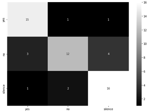 Figure 5: example confusion matrix. The y axis shows the true labels while the x axis shows predicted labels.
In this example we have a high number (4) of ‘no’ utterances being classified as silence. That can systematically be investigated now.
Exercise time: Now is a great time to complete exercise 2 before the next part of the article.
Part 2a: Common problems and solutions
At the end of exercise 2 we encountered a problem called overfitting, which manifested itself in the gap between train and test accuracy. Another typical problem is called underfitting, which itself can be seen by a model not even producing good training accuracy. Schematically, what happens is shown below:
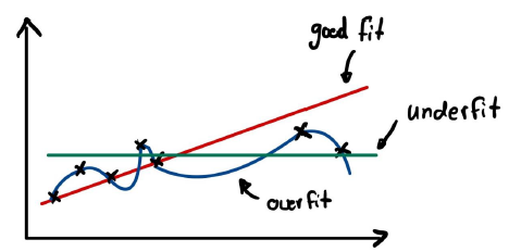 Figure 6: over and underfitting
The green curve is obviously not powerful enough to capture the variation in the data. It is very biased in assuming that the slope of the curve that describes the data is zero. In contrast, the blue curve is reproducing the data perfectly, however it does not capture the trend of increasing y values for increasing x values at all. The blue model has a low bias (aka many parameters) and learns the random fluctuations in the data instead of capturing the general trend. This is a problem of all supervised learning algorithms, and it is called the Bias-variance tradeoff. One would ideally have a model with just the right amount of bias, just like the red curve in our example. There are techniques to deal with both over- and underfitting. Let’s look at underfitting first.
The easiest way of dealing with underfitting is to use a more powerful model. For neural networks this usually means more parameters. But one can also fight it by using a model or features that are more tailored to the problem as the following example illustrates:
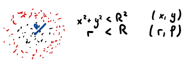 Figure 7: some parameters are better than others for a given classification problem.
The red points have a distance larger than R from the center. The function that we look for here can be parameterized by one variable (r) if chosen wisely. Alternatively, one can use the two variables x and y to describe the function. An algorithm using only x as a parameter would not have been able to describe the data (underfitting).
Overfitting can firstly be tackled by using models with less parameters, as is obvious from our example. Reducing the noise within the dataset can help, as well as stopping the training early. It is also common to reduce the degrees of freedom using some or all the following regularization methods:
-
Weight penalty
-
Dropout
-
Batch normalization
-
Data augmentation
Weight penalty
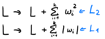
The idea is to add a term to the loss function that is related to the size of the weights. This provides an incentive to make unimportant weights small.
 Equation 4: weight penalty examples.
The most common form is L2 regularization, as shown above. In practice one can configure this layer wise in deep learning frameworks like Keras, to add only some terms to the loss.
Dropout
The idea is that neurons randomly drop out of the training, effectively training an ensemble of models with shared weights. See this paper for details.
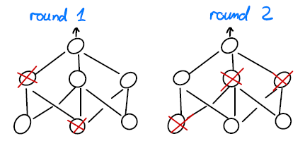 Figure 8: dropout example.
The dropout probability is set to 0 when the model is used for inference.
Batch normalization
Batch norm layers are used to normalize the input to zero mean and unit variance. That improves the training for several reasons, and it is often used in multiple points in the network. Since the training is usually done in batches, it is not clear what the mean and variance of the training set are at a given point in the network and given time during training. Therefore, Batch normalization uses all data points in the training batch for a component wise optimization. Detail can be found here.
Data augmentation
Having more (quality) data can also prevent overfitting. Imagine in our example in Figure 6 we had also data points in the mid x region and more data points overall. That might have allowed our blue curve to catch the general trend after all. While the other methods we introduced are relatively easy modifications of the model or training algorithm, it is usually harder to get new data. It is, however, possible to use the data we have to create new data, via:
-
varying data quality (e.g., resolution)
-
varying experimental conditions (e.g., lighting)
-
applying various other symmetry operations that the network should learn (e.g., rotations)
Regarding audio data we can use augmentation before feature extraction, e.g., we can adjust:
-
Pitch
-
Speed
-
Amplitude
-
background noise and noise levels
It is also possible to apply data augmentation to the spectrograms, like:
-
cover random parts of the spectrogram (see this paper)
-
translation along the time axis
Part 2b: Improving the model architecture
It is time to improve the architecture of the neural network to obtain better results in terms of performance and network efficiency. We have already discussed that the spectrograms can be seen as a grayscale image. Hence, we can borrow ideas from image classification tasks, one of which are Convolutional Neural Networks (CNNs).
Convolutional Neural Network (CNN)
CNNs are much more efficient in terms of their network structure than FFNNs when it comes to e.g., image processing tasks. They impose translation invariance on the network structure itself. This is done by using the same set of weights over the whole image, regardless of the position. Here is the comparison of a FNN and a CNN in a simplified view:
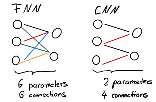 Figure 9: FFNN vs. CNN. colors are weight values.
The Figure shows that CNN layers do not just connect every neuron with every other neuron but use the same parameter values for the weights over the entire input. That reduces both the number of connections in the network as well as the number of free parameters of the model.
An intuitive understanding of a CNN layer is presented on this website and most easily understood by considering classical image processing. Suppose one has a grayscale image of size (TxF) pixels and wants to find edges in the image. Then one would apply a filter to obtain the new image with just the edges of the objects in it.
 Figure 10: gradient like filter applied to the input image.
Mathematically this means using a kernel to obtain a pixel in the new image as a weighted sum over the original pixel and its neighbors. In the example above we used the following kernel:
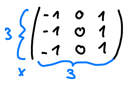 Figure 11: kernel applied in Figure 10.
The example above is a 2D kernel of size 3 and it has a receptive field of 3x3 pixels, 3 in x and 3 in y direction.
Many operations like edge finding can be described using different kernels. In a convolutional layer the weights of the kernel are learned and hence many different filters can be learned by the network, depending on the needs for the task. In fact, a convolutional layer usually learns multiple filters. Output images of such a layer are called feature maps. Naturally, the size of a feature map is different from the size of the input the kernel operates on. Let’s take on the model builders’ perspective. We might want to achieve:
-
the same size of input and feature map
-
a smaller feature map size compared to the input
The former can be achieved by adding a frame of 0’s to the original image to artificially enlarge it and consequently the feature map size. This is called padding. The latter can be achieved by introducing strides or pooling. Strides is increasing the hop size when applying the filter from its default (one) to s, whereas pooling summarizes a group of pixels in a feature map to one value, e.g. via taking the maximum. A great visualization of the effect of parameters like stride can be found here and a great visualization as well as the mathematical formula in chapter 14, here.
Let’s go back to our keyword spotting project. Since the structure of the network input (MFCC features) is similar to a grayscale image, we can use various CNN models that work well for image classification. A selection of ready to use Keras models can be found here. We will use one of the readily available models in the exercises as well.
Further improving the architecture
Another approach is to search the literature for available models that fit our needs. One such model is the TC-ResNet. It is suitable for our purpose, since it is very small footprint and relatively easy to implement.
residual networks
A common trick is to use residual connections. The idea is to have two paths in the network graph, one passes on the input, the second one learns weights. The result of both paths is then added up.
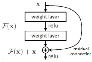 Figure 12: residual connections. Figure from He et. al 2016.
These residual networks (ResNets) help to achieve deeper network architectures and are quite popular.
TC-ResNet
The TC-ResNet was originally proposed here. The thought process is the following: Consider the MFCC features to be a time series with T elements of F images, each of dimension one. So instead of our (TxFx1) dimensional grayscale image we have a (Tx1xF) series of F, one-dimensional images, one for each MFCC coefficient. A convolutional kernel can now be applied that simultaneously goes over all F images. That means that even the first convolutional layer already has access to all frequencies, whereas using 2D convolutions on a (TxFx1) grayscale image the first kernel only has access to some frequency values at a time.
.](/assets/img/1*F2U-sEOcxm9QWk0IMjrf_Q.png) Figure 13: idea (left) and network structure (right) of the TC-ResNet. Taken from Choi et. al, here.
Figure 13: idea (left) and network structure (right) of the TC-ResNet. Taken from Choi et. al, here.
The architecture further makes use of residual blocks (blue). These tricks allow for an architecture with less than 100k parameters that is working well for our task. This is however not the only small footprint architecture. More can be found here.
Exercise time: Now is a great time to complete exercise 3!
Wow! That’s it! We have trained a neural network for classifying keywords that works. We are ready to try it out in the next and last part of the tutorial.
Please get in touch with your questions, suggestions, and feedback!
Further resources:
-
He, Kaiming, et al. “Deep residual learning for image recognition.” Proceedings of the IEEE conference on computer vision and pattern recognition. 2016.
-
Hinton, Geoffrey E., et al. “Improving neural networks by preventing co-adaptation of feature detectors.” arXiv preprint arXiv:1207.0580 (2012).
-
Zhang, Yundong, et al. “Hello edge: Keyword spotting on microcontrollers.” arXiv preprint arXiv:1711.07128 (2017).
-
Warden, Pete. “Speech commands: A dataset for limited-vocabulary speech recognition.” arXiv preprint arXiv:1804.03209 (2018).
-
Choi, Seungwoo, et al. “Temporal convolution for real-time keyword spotting on mobile devices.” arXiv preprint arXiv:1904.03814 (2019).
-
Park, Daniel S., et al. “Specaugment: A simple data augmentation method for automatic speech recognition.” arXiv preprint arXiv:1904.08779 (2019).
-
Géron, Aurélien. Hands-on machine learning with Scikit-Learn, Keras, and TensorFlow: Concepts, tools, and techniques to build intelligent systems. “ O’Reilly Media, Inc.”, 2019.