Speech recognition 101: Hands on Keyword Spotting 3/3
This 3-part tutorial series will take you on an adventure to build your own neural network keyword spotter with step-by-step lecture and coding exercises. In part three we will build a small app to deploy and play with our keyword spotter.
 source: pixabay
The tutorial series
Recognizing speech is one of the most prominent audio tasks and it can be quite complex to design Automatic Speech Recognition (ASR) systems usually requiring expert knowledge, large datasets and computational resources. Consequently, the topic is hard to access for beginners. Keyword Spotting is the task of recognizing a set of keywords from an audio stream or file and good models can be trained with fewer data, less computing time and conceptual difficulty. Therefore, it is the ideal starting point for learners and we will build a keyword spotter from scratch, in the following three tutorials:
-
Audio: preprocessing data for speech recognition tasks
-
Machine Learning: training neural networks for keyword spotting
-
Application: Building an app to deploy the model in a Jupyter Notebook
The code and exercises were designed for the audio track of ML summer school and every article will have theory input followed by practical exercises, that can be downloaded from this repository.
The big picture
The big picture of the keyword spotter is shown below. We have dealt with the Feature Extractor, trained a classifier and will now build a post processor and put everything together.
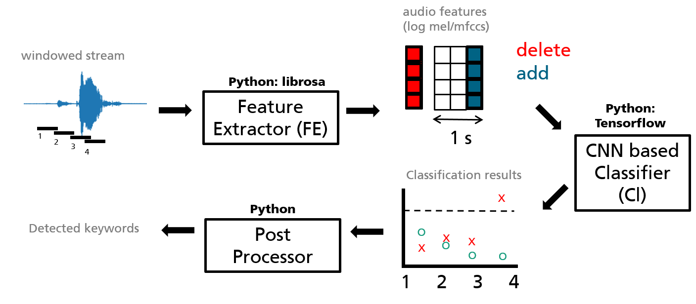 Figure 1: big picture of the keyword spotting application.
Post Processor
The post processor is the last puzzle piece we need to build. Its purpose is to interpret the classifier’s output and tell us when a keyword was detected and which one it was. We do this by processing the classifier’s output in two steps:
-
we average over the last couple of classifier outputs. This is analogue to smoothing the probabilities that are sent over by the classifier
-
we set a threshold for the smoothed probability. If it is crossed, the post processor will tell us it found a keyword
Streaming
How does the whole application come together now? The whole process is shown in Figure one. Let’s go through it again, step by step.

The microphone sends a chunk of audio (black horizontal lines) to the feature extractor. It extracts and returns feature vectors, one for each chunk. The feature vectors are aggregated until a length of one second is achieved. (Three vertical bars in the Figure). If we already have the equivalence of one second of audio data gathered, we delete the oldest feature vector from the left and add the latest feature vector to the right. The result is an image of feature vectors (MFCCs) that gets updated always after a new chunk of audio has been processed.
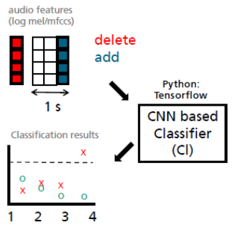
The image is sent to the classifier. We have designed the **classifier **in such a way, that it returns class probabilities, where every class corresponds to a keyword (yes, no, …) or one of the non-keyword classes: silence and unknown. The classifier is applied whenever an updated image comes in (it could also use a different frequency, but it is easier for now to do it that way). Therefore, each audio chunk returns a probability vector after it has passed through the feature extractor and the classifier. The result is scratched in Figure one: We obtain a series of class probabilities. In the Figure red and green stand for probabilities of different keywords (they should add up to one).

The post processor is then applied whenever a new probability output comes in (again it could be applied at a different frequency, but it is easier for now). Let’s say the smoothing operation takes the element wise average over the last three probability vectors. The result is a smoothed probability curve that lags by three audio chunks compared to the non-smoothed curve. It is smoothed since a keyword probability must be high over multiple audio chunks to be high in the averaged probability vector. That makes it much more suitable to operate on. Whenever one class probability crosses the predefined threshold, the post processor will fire and tell us it has detected the corresponding keyword.
Let’s go to exercise 4!
That’s it! We have all ingredients to build the keyword spotter. Thanks a lot, you have taken the journey with me. I am looking forward to your** comments and feedback**. Have fun now putting everything together and playing with your own keyword spotter.
Further reading:
-
Chen, Guoguo, Carolina Parada, and Georg Heigold. “Small-footprint keyword spotting using deep neural networks.” 2014 IEEE International Conference on Acoustics, Speech and Signal Processing (ICASSP). IEEE, 2014.
-
Sainath, Tara, and Carolina Parada. “Convolutional neural networks for small-footprint keyword spotting.” (2015).
-
Rybakov, Oleg, et al. “Streaming keyword spotting on mobile devices.” arXiv preprint arXiv:2005.06720 (2020).