Speech recognition 101: Hands on Keyword Spotting 1/3
This 3-part tutorial series will take you on an adventure to build your own neural network keyword spotter with step-by-step lecture and coding exercises. Part one will discuss the processing of speech data.
 source: Pixabay
The tutorial series
Automatic Speech Recognition (ASR) is the task of translating speech to text. A full fetched ASR system is very powerful and has a wide range of applications. However, building such systems usually requires expert knowledge, large datasets and computational resources. Consequently, the topic is hard to access for beginners. Meanwhile Keyword Spotting (KWS) is the task of recognizing a limited set of keywords from speech. While conceptually similar, building decent models requires less data, computing time and less expert knowledge. Therefore, it is the ideal starting point for learners and we will build a keyword spotter from scratch, in the following three tutorials:
-
Audio: preprocessing data for speech recognition tasks
-
Machine Learning: training neural networks for keyword spotting
-
Application: Building an app to deploy the model in a Jupyter Notebook
The code and exercises were designed for the audio track of ML summer school at University of Cologne and every article will have theory input followed by practical exercises, that can be downloaded from this repository.
The big picture
The big picture is shown below and will make sense over the cause of the series.
 Figure 1: Overview of the keyword spotting app
We start on the left with the raw audio signal and end up with a detected keyword on the very end of the pipeline. There are roughly three parts of the keyword spotter: Feature extractor, classifier and post processor. We will discuss the Feature Extractor in the following.
Audio 1a: preprocessing data for speech recognition tasks
What is audio data?
Audio in general and speech in particular can be understood as a series of amplitude values over time, see Figure 2. The speech samples are usually sampled equidistantly. The dataset we use stores this amplitude information in .wav files and the data are recorded with a frequency of 16 kHz, meaning that the amplitude values are recorded 16.000 times per second. We call this series ‘a’ and it’s length ‘N’.
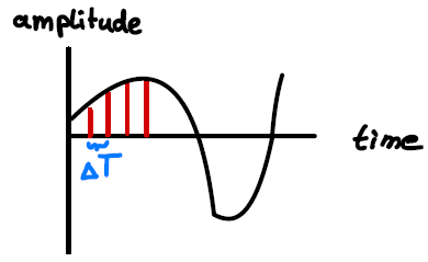 Figure 2: An audio signal is sampled over time
While many modern speech recognition models learn the feature extraction themselves, it is still useful to perform manual feature extraction. A useful representation of an audio signal can be obtained by applying the Short Time Fourier Transformation (STFT), which is an application of the Discrete Fourier Transform (DFT) to short, consecutive parts of the signal. DFT itself is the discrete version of the famous Fourier Series.
Fourier Series
The Fourier Series expands a periodic function in terms of a sum of sin and cos functions. An example is shown below. We can see that the original function (black curve) is already approximation well by a few terms (red curve). The second term has a frequency of 3 and a coefficient of 1/3 and so on.
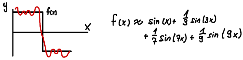 Figure 3: Approximation of a step function (black curve) using the Fourier Series f(x) (red curve).
While this can be applied generally, it is useful for sound, since the expansion is packed with physics. Sin and cos terms correspond to different frequencies in the signal, while the coefficients in front of them are related to the energy stored in that frequency.
Discrete Fourier Transform (DFT)
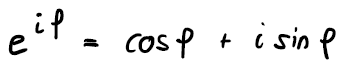
The DFT decomposes a sequence of values into a finite sum of sin and cos functions. Instead of sin and cos, the DFT can also be written as a sum of exponential functions with potentially complex coefficients. This exponential notation is more compact then using sin and cos terms, but there is a one-to-one relationship via Euler’s Formula:
This is more compact and is shown in the first row below:
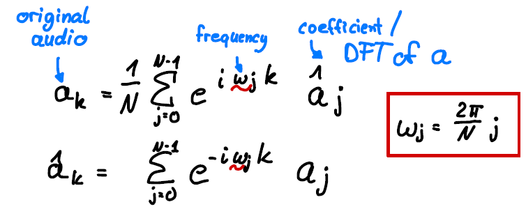 Equation 1: Relation between DFT and inverse DFT coefficients
The coefficients of that expansion which are also called the DFT of the signal, can be obtained as shown in the second row. Here a is the series in the time domain and hatted a’s are the coefficients/DFT of the series in frequency domain. The absolute value of the coefficients is related to the energy stored in the accompanying frequency.
Short Time FT (STFT)
Now we are equipped with the tools to go back to our audio signal. To understand the time dependence of the frequencies in the signal, one can apply the discrete Fourier transform to consecutive, potentially overlapping segments of the signal in the time domain. This is called Short Time Fourier Transform (STFT). It is done by applying the DFT on L samples of the signal at a time, where L is chosen to correspond to a small-time interval, e.g. the amount of samples corresponding to 40 ms. (In our example with a sample frequency of 16 kHz this would be L=640 samples). The next application of DFT starts H (hopping size) samples later. Usually H<L, which means there is a stride (overlap) of S samples between consecutive windows.
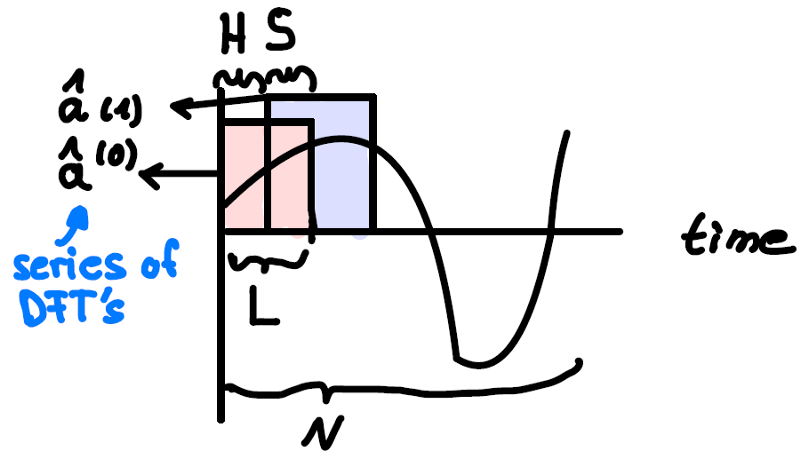 Figure 4: STFT applied to an audio signal of N samples with window length L, hopping size H and stride S. Two DFT applications are shown.
The smaller we choose L, the better the time resolution gets. This comes at a cost: Smaller L’s mean less terms in the corresponding DFT series in equation 1, meaning we have a worse frequency resolution. (Note that the frequencies go with 1/N which is L in the case of STFT).
The result of each DFT is a vector with potentially complex coefficients of the frequencies in the signal, as was shown in Figure 4. Consequently, the result of the STFT is a time series of such vectors. Let’s call the number of times we apply DFT M and put the vectors we get from DFT into the rows of a matrix. That matrix has M columns, corresponding to the M times we applied the DFT on the time axis and F rows, one for each coefficient obtained from applying the DFT. After squaring each value, it looks like this:
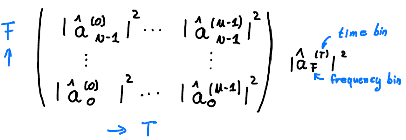 Figure 5: STFT coefficients in matrix form constitute a spectrogram.
We square the values since only the absolute value of the potentially complex coefficients is of interest. If we plot it, we get a so-called spectrogram. The colors show how much energy is stored in which frequency bin at a given time bin T. That provides a human readable form of the signal. For example, a vowel will show up as a horizontal line (fixed frequency) in such a spectrogram.
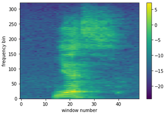 Figure 6: spectrogram of the word “yes”. We took the log of the coefficients for better visibility.
This is great! We have a human readable, more compact form of the signal. In the following we will make some improvements, but the hardest part is over.
MEL Spectrogram
It is known that the human ear (which is a great tool for speech recognition) perceives frequencies in a non-linear fashion. It is very good at distinguishing small differences of small frequencies, while small differences at big frequencies sound very similar to us. Therefore, it is good practice to transform the frequency axis according to the MEL scale:
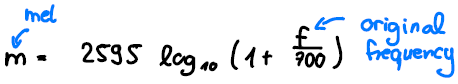 equation 2: Mel scale.
In practice we apply several triangular filters equidistantly to the MEL scaled frequency axis and thereby obtain a value for each of the applications of the filter. Doing this, we look closer at smaller frequencies, where the interval is small and have a rougher look at bigger frequencies, where the filter covers a large frequency interval. This is illustrated in the following diagram.
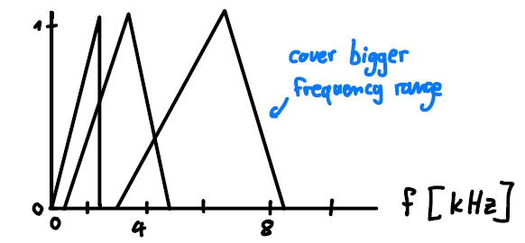 Figure 7: Mel filter bank.
In the illustration we use 3 filters only. Usually, more filters are used, e.g. 13. Furthermore, we want to take the logarithm of the coefficients as well. This is motivated by the non-linear human perception of loudness. The result is called the log-MEL spectrogram. It is tailor made for speech recognition tasks. Here is an example of the word yes:
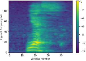 Figure 8: log MEL spectrogram of the word yes.
We can see that the lower frequency bins are much more pronounced when we compare to Figure 7. This is exactly what we wanted. While this can be used for speech recognition tasks perfectly well, there is an additional step we want to take.
MFCC features
Creating speech is basically a two-stage process. There is a source, which is a stream of air from your lungs that triggers a vibration of the vocal folds. The resulting source signal is then filtered by our vocal tract to create the final speech signal.
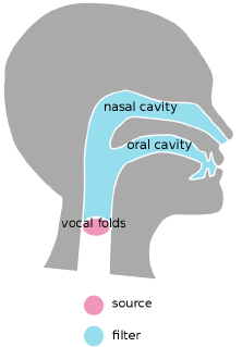 Figure 9: Speech generation. Emflazie, CC BY SA 4.0 https://creativecommons.org/licenses/bysa/4.0, via Wikimedia Commons
While the source part is useful to characterize who is speaking the filter part is relevant for what has been said. Therefore, for speech recognition, we want to isolate it from the rest of the signal and the mathematical way of doing this is to transform the log MEL spectrogram with the discrete cosine transformation back to the time domain. This works because the product of source and filter can be decomposed by STFT, logarithm and discrete cosine transform, in that order. The resulting coefficients are called Mel Frequency Cepstral Coefficients or MFCCs.
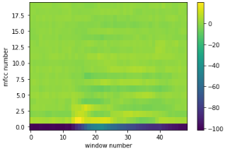 Figure 10: MFCC coefficients for the spectrograms shown above.
Summary
We have learned how to extract speech features from audio signals. The pipeline is the following:
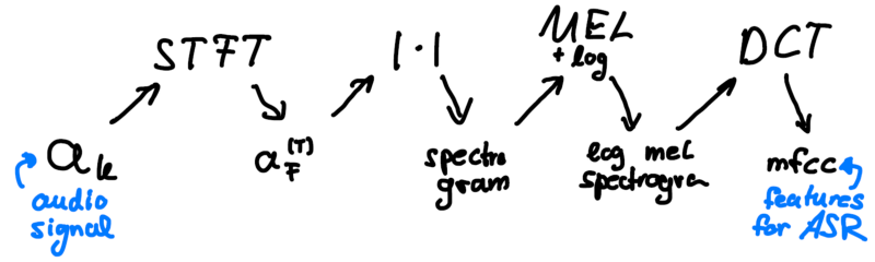
That’s all! We have a great set of features for our speech signal and are now ready to get our hands dirty and play around with what we just learned.
Audio 1b: preparing data for increased robustness
To improve the robustness and overall performance of speech recognition models, it is a vital step to use data augmentation. This does two things at once. Firstly, it increases the dataset size, supporting neural network training. Secondly, it can be used to present data with recording conditions that match the deployment conditions of the model in the real world, increasing robustness.
There are a variety of methods available, whose success depends on the Use Case at hand. Problems can be reverberation, specific background noise, insufficient speaker loudness etc. But the idea is always the same: We will create samples with these conditions from samples within our training data. In the exercises we will look at two specific methods: Time Shift, corresponding to keywords being recorded only partially and the addition of background noise. We will discuss this in more depth in the next article.
Let’s go to exercise 1. It’s worth checking it out to get a deeper understanding of what we have discussed!
Please get in touch with your questions, suggestions and feedback!
Further Resources
-
See this video for a more in-depth visual introduction to the Fourier Transform.
-
The University of Edinburgh University ASR lecture notes provide a great resource for learning more about ASR.
-
Oppenheim, Alan V., John R. Buck, and Ronald W. Schafer. Discrete-time signal processing. Vol. 2. Upper Saddle River, NJ: Prentice Hall, 2001.
-
More on feature extraction can be found here.